OpenPano: How to write a Panorama Stitcher
This is a summary of the algorithms I used to write OpenPano: an open source panorama stitcher. You can find the source code on github.
SIFT Feature
Lowe's SIFT [1] algorithm is implemented in feature/.
The procedure of the algorithm and some results are briefly described in this section.
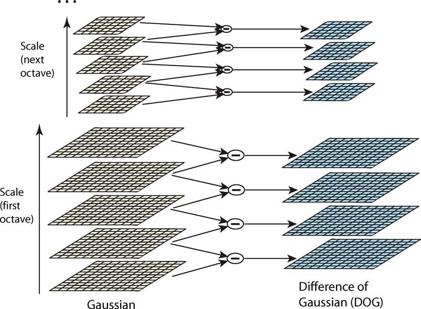
Scale Space & DOG Space
A Scale Space consisting of
The gaussian blur here is implemented by applying two 1-D convolutions, rather than a 2-D convolution. This speeds up the computation significantly.
In each octave, calculate the differences of every two adjacent blurred images, to build a Difference-of-Gaussian space.
DOG Space consists of
Extrema Detection
In DOG Space, detect all the minimum and maximum
by comparing a pixel with its 26 neighbors in three directions:
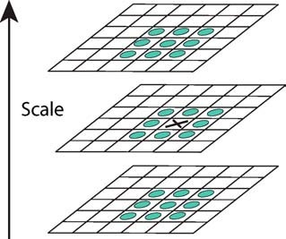
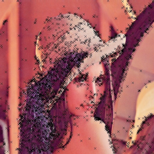
Then use parabolic interpolation to look for the accurate

Orientation Assignment
First, we calculate gradient and orientation for every point in the Scale space. For each keypoint detected by the previous procedure, the orientations of its neighbor points will be collected and used to build an orientation histogram, weighted by the magnitude of their gradients, together with a gaussian kernel centered at the keypoint. The peak in the histogram is chosen to be the major orientation of the keypoint, as shown by the arrows below:

Descriptor Representation
Lowe suggested [1] choosing 16 points around the keypoint, to build orientation histograms for each point and concatenate them as SIFT feature. Each histogram uses 8 different bins ranging from 0 to 360 degree. Therefore the result feature is a 128-dimensional floating point vector. Since the major orientation of the keypoint is known, by using relative orientation to the major one, this feature is rotation-invariant.
Also, I followed the suggestions from [2] to use RootSIFT, which is a simple modification on SIFT, and is considered more robust.
Feature Matching
Euclidean distance of the 128-dimensional descriptor is the distance measure for feature matching between two images. A match is considered not convincing and therefore rejected, if the distances from a point to its closest neighbor and second-closest neighbor are similar. A result of matching is shown:
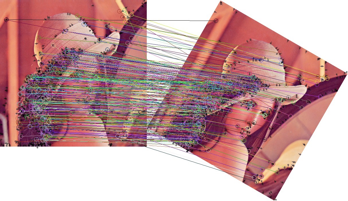
Feature matching turned out to be the most time-consuming step. So I use FLANN library to query 2-nearest-neighbor among feature vectors. To calculate Euclidean distance of two vectors, Intel SSE intrinsics are used to speed up.
Transformation Estimation
Estimate from Match
It's well known [3] that
for any two images taken from a camera at some fixed point,
the homogeneous coordinates of matching points
can be related by a homography matrix
Homography I:
Homography II:
When two images are taken with only camera translation
and rotation aligned with the image plane (no perspective skew),
then they can be related by an affine matrix of the form:
Given a set of matches, a matrix of any of the above formulations
can be estimated via Direct Linear Transform.
These estimation methods are implemented in lib/imgproc.cc. See [3] for details.
However these methods are not robust to noise.
In practice, due to the existence of false matches,
RANSAC (Random Sample Consensus) algorithm [4] is used to estimate a transformation matrix
from noisy data.
In every RANSAC iteration, several matched pairs of points are randomly chosen to produce a best-fit transformation matrix,
and the pairs which agree with the matrix are taken as inliers.
After a number of iterations, the transform that has most number of inliers are taken as the final result.
It's implemented in stitch/transform_estimate.cc.
Match Validation
After each matrix estimation, I performed
a health check to the matrix,
to avoid malformed transformation
estimated from false matches.
This includes two checks: (see stitch/homography.hh)
-
The skew factor in homography (
-
Flipping cannot happen in image stitching. A homography is rejected if it flips either
In unconstrained stitching, it's necessary to decide whether two images match or not. The number of inliers estimated above could be one criteria. However, for high-resolution images, it's common that you'll actually find false matches with a considerable number of inliers, as long as enough RANSAC iterations are performed. To solve this, note that false matches are usually more randomly distributed spatially, geometry constraints of matching can also help filter out bad matches. Therefore, after RANSAC finished and returned a set of inliers, some overlapping test can be used to further validate the matching, as suggested by [5].
Specifically, with a candidate transformation matrix, I could find out the region within one image covered by another image, by calculating the convex hull of the transformed corners. Two filters can then be applied after the overlapping region is found:
- The overlapping area within two images shouldn't differ too much.
- Within the region, a reasonably large portion of matches should be inliers. I also used the inlier ratio as the confidence score of this match.
Since false matches are likely to be random and irregular, this technique help filter out false matches with irregular geometry.
Cylindrical Panorama
Necessity of Projection
If a single-direction rotational input is given, as most panoramas are built, using planar homography leads to vertical distortion, as following:
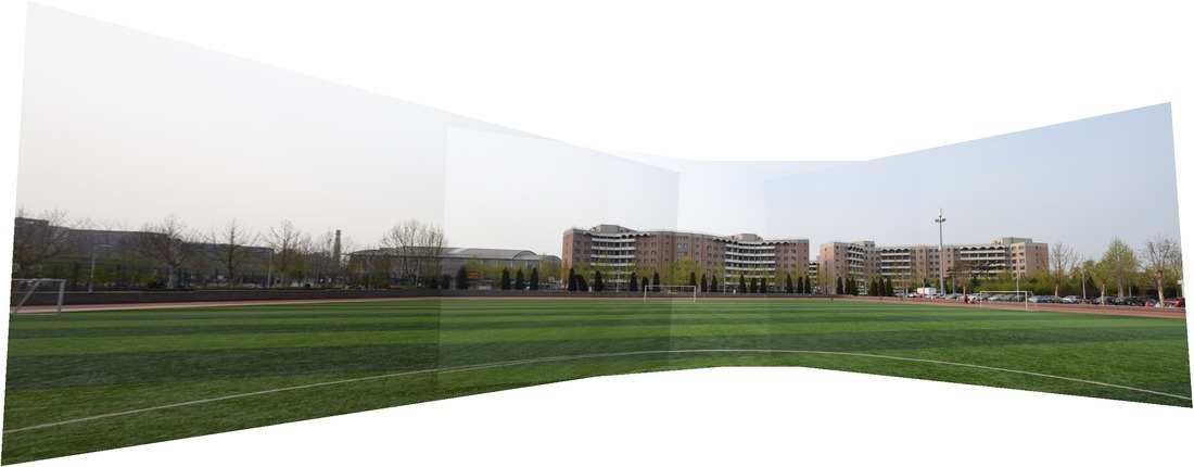
This is because a panorama is essentially an image taken with a cylindrical or spherical lens, not a planar lens any more. Under this setting, the white circle on the grass around the camera (as in the above picture) is expected to become a straight line. A good demo revealing the reason of this projection can be seen at this page.
The way to handle this problem is to warp images by a cylindrical or spherical
projection, before or after transform estimation.
These are the two modes used in this system. In this section we will
introduce the pipeline based on pre-warping, which is used in cylinder mode. This pipeline is
generally good, although it has more assumptions on the data and requires some tricks to work well.
It is implemented in stitch/cylstitcher.cc.
Warp
We can project the image to a cylinder surface at the beginning of stitching, by the following formula:
stitch/warp.cc. Some example images after warping
are given below. Note that this requires focal length to be known ahead of time, otherwise
it won't produce a good warping result.
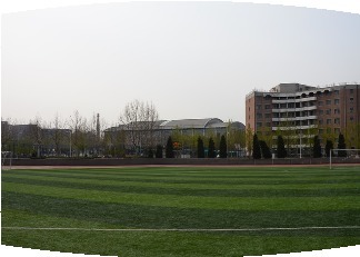
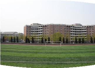
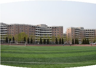
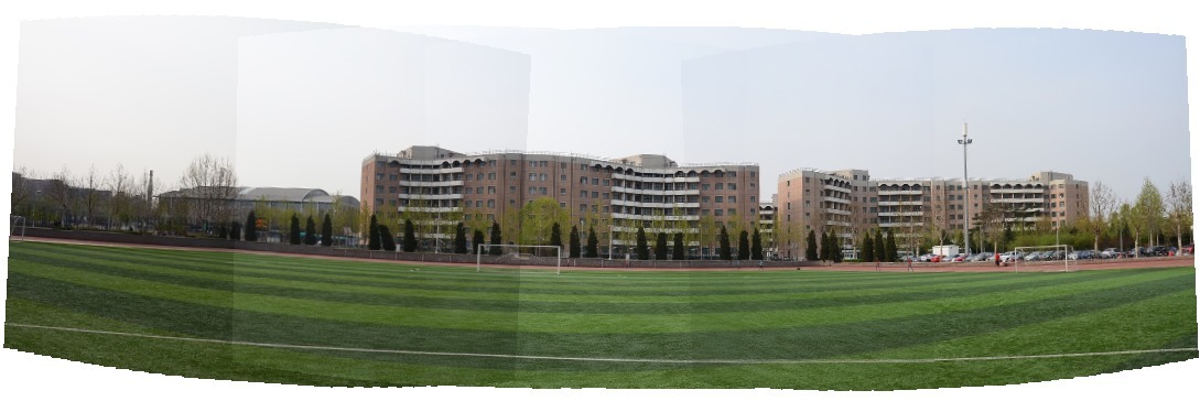
After projecting all images to the same cylinder surface, images can be simply stitched together by estimating pairwise affine transformation, and accumulating them with respect to an arbitrarily chosen identity image. Note that the white line on the ground is more straightened.
Straightening
The cylinder projection equations described above assumes horizontal cameras (i.e. only 1 DOF is allowed for the relative rotation between cameras). This assumption could lead to distortion, then the output panorama would be bended:

Choosing the middle image as the identity help with this problem.
Another method I found to effectively reduce the effect is to searching for
Since the effect is caused by camera tilt,

The change of

Camera Estimation Mode
Intuition
Cylinder mode assumes a known focal length and requires all cameras to have the same "up" vector, to warp them on cylinder surface at the beginning. We want to get rid of these assumptions.
However, if you simply estimate pairwise homographies, directly stitch them together, and perform a cylindrical warp after the transformation (instead of before), you'll get something like this:

Notice that images indeed are well stitched together: matched points are overlapped very well. But the overall geometry structure is broken.
This is because
Also, we noticed that
This inconsistent over-parameterization of camera parameters can lead to the kind of overfitting results above, that breaks the underlying geometry structure.
People use
Initial Estimation
[6] gives a method to roughly estimate the focal length of all images at first. Given all focal length and
the rotation matrix of one image, the rotation matrix of a connecting image can be estimated by
using the homography we already have:
Therefore, the estimation procedure goes like a max-spanning tree algorithm: after building a pairwise-matching graph,
I first choose an image with good connection property to be identity.
Then, in each step a best matching image (in terms of matching confidence) not processed yet is
chosen and its rotation matrix stitch/camera_estimate.cc.
Note that, since the homography
If no bundle adjusment is performed,
the stitching result will misalign and looks like this, due to wrong formulation of

To further refine the parameters in
Bundle Adjustment
We setup a consistent parameterization of
Iterative methods such as Newton's method, gradient descent,
and Levenberg-Marquardt algorithm can be used to
solve the optimization.
Assume matrix
- Gradient descent:
- Newton's method:
- LM algorithm:
All iterative methods involve calculating the matrix
-
Numeric: For each parameter
-
Symbolic: Calculate
The last equation is from the result of [7].
By the way, it's interesting to point out that Lowe's paper [5] actually gives an incorrect formula:
Both methods are implemented in stitch/incremental_bundle_adjuster.cc.
Symbolic method is faster because it allows us to calculate only those
non-zero elements in the very-sparse matrix
In a collection of
After optimization, the above panorama looks much better:

Straightening
Straightening is necessary as well.
As suggested by [5], the result of bundle adjustment
can still have wavy effect, due to the tilt angle ambiguity.
By assuming all cameras have their
See the following two images and notice the straight line on the grass is corrected (it is actually a circle in the center of a soccer field).


Blending
The size of the final result is determined after having all the transformations. And the pixel value in the result image is calculated by an inverse transformation and bilinear interpolation with nearby pixels, in order to reduce alias effect.
For overlapped regions, the distance from the
overlapped pixel to each image center is used to calculate
a weighted sum of the pixel value.
I only used the distance along the
Cropping
When the option CROP is given,
the program manages to find the largest valid rectangular within the original result.
An
For each row


[1]: Distinctive Image Features From Scale-invariant Keypoints, IJCV04
[2]: Three Things Everyone Should Know to Improve Object Retrieval, CVPR2012
[3]: Multiple View Geometry in Computer Vision, Second Edition
[4]: Random Sample Consensus: a Paradigm for Model Fitting with Applications to Image Analysis and Automated Cartography, Comm of ACM, 1981
[5]: Automatic Panoramic Image Stitching Using Invariant Features, IJCV07
[6]: Construction of Panoramic Image Mosaics with Global and Local Alignment, IJCV00
[7]: A Compact Formula for the Derivative of a 3-D Rotation in Exponential Coordinates, arxiv preprint
BTW, you can download these papers with my automatic paper downloader:
pip install --user sopaper
while read -r p
do
  sopaper "$p"
done <<EOM
Distinctive Image Features From Scale-invariant Keypoints
Three Things Everyone Should Know to Improve Object Retrieval
Random Sample Consensus: a Paradigm for Model Fitting with Applications to Image Analysis and Automated Cartography
Automatic Panoramic Image Stitching Using Invariant Features
Construction of Panoramic Image Mosaics with Global and Local Alignment
A Compact Formula for the Derivative of a 3-D Rotation in Exponential Coordinates
EOM