Where Are Pixels? -- a Deep Learning Perspective
Technically, an image is a function that maps a continuous domain, e.g.
a box array[H][W], where each element
array[i][j] is a pixel.
How does discretization work? How does a discrete pixel relate to the abstract notion of the underlying continuous image? These basic questions play an important role in computer graphics & computer vision algorithms.
This article discusses these low-level details, and how they affect our CNN models and deep learning libraries. If you ever wonder which resize function to use or whether you should add/subtract 0.5 or 1 to some pixel coordinates, you may find answers here. Interestingly, these details have contributed to many accuracy improvements in Detectron and Detectron2.
Formation of Discrete Image
Sampling theory tells us how a continuous 2D signal is turned into a discrete array by sampling and filtering.
-
We choose a
rectangular grid of points, from which we will draw samples. In order to make the best use of the produced samples, we have to know the exact location where every sample on this grid is chosen. -
Values on these sampled points are not directly retrieved from the original signal, but come from a filtering step that removes high-frequency components. A bad choice of filters can lead to aliasing effects.
Sampling and filtering are both important in basic image processing operations, such as resize. Resize operation takes a discrete image, resamples it, and creates a new image. The choice of sampling grid and sampling filter will then affect how such a basic operation is implemented.
For example, the paper On Buggy Resizing Libraries and Surprising Subtleties in FID Calculation studies the filtering issues, and shows that the resize operations in many libraries (OpenCV, PyTorch, TensorFlow) don't take into account the low-pass filtering. This then leads to incorrect deep learning evaluation.
In this article, we ignore the issue of sampling filter, and only study the coordinates of sampling grid. We'll see that this choice is also inconsistent among libraries, and can affect the design and performance of CNN models.
Choices of Sampling Grid
Pixels are located on a sampling grid we choose. Naturally, we would like to only consider rectangular grids where pixels are spaced evenly. But there are many other factors to be concerned with:
- Offset: where is the first pixel located relative to the beginning of the signal?
- Stride: what's the distance between two neighboring pixels?
- Resolution: how many pixels are there?
(These terminologies may have a different meaning elsewhere, but this is how I define them in this article.)
For simplicity, we look at the one-dimensional case instead.
We want to answer this question: for a 1D signal defined on
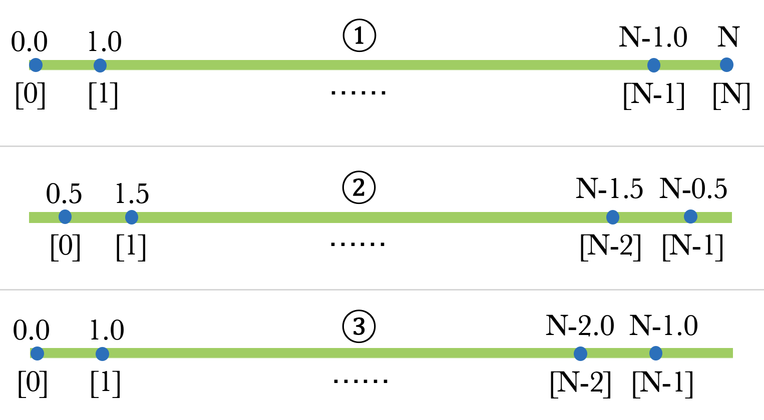
In this figure, the green bars represent the 1D signal of length
They (or at least the first two) are all valid interpretations when we are given an array of pixels. The interpretation we choose affects how we implement operations and models, because they each have some unique weird properties. To understand them more, let's check how a 2x resize operation should be implemented under each interpretation.
2x Resize Operation
We'll now see that a simple "2x resize" operation has many possible implementations.
A unique undesired property of ① is that, stride is not the inverse of resolution. So a 2x resize is ambiguous: we have to be clear about whether we want half of stride, or twice more pixels. The new grids after resize look like these:
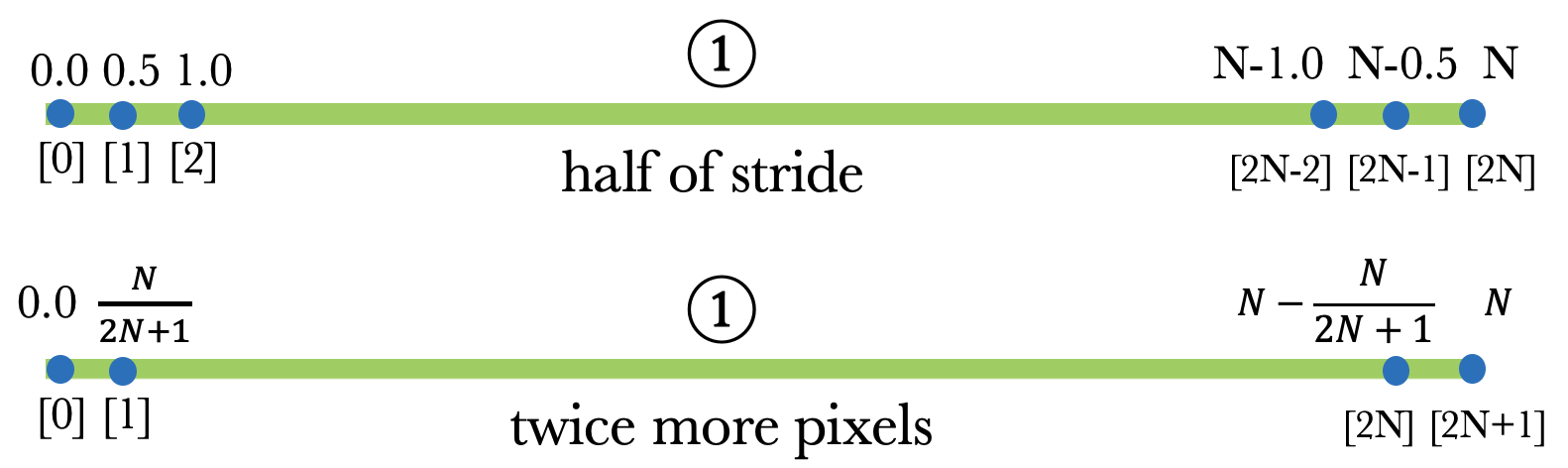
Resize for grid ② & ③ aren't ambiguous:
You can easily verify that the 4 different resized grids still match the corresponding definition in our table above.
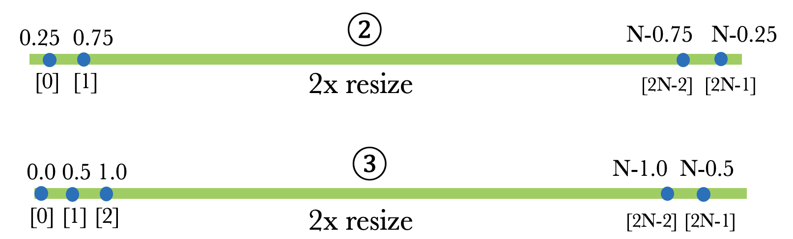
For 2D case, the 2x resize in ①(twice more pixels) and ② look liks this (image credit: here),
from which you can see why ①(twice more pixels) is also called align_corners:
These 4 different versions of 2x resize have some issues:
-
Extrapolation: ② and ③ both need extrapolation outside the border of the original grid to perform resize, but ① only needs interpolation. Extrapolation is sometimes undesirable.
-
Asymmetry: ③ is asymmetric, and it's probably a good reason to never use it. One consequence is that
resize(flip(x)) != flip(resize(x)). All others are symmetric. -
Information Loss: in ①(half of stride) and ③ , about half of the points on the new grid exist in the old grid. By not having to interpolate their values, we minimize the loss of information. However, in ①(twice more pixels) and ②, most or all of the new pixels need to be recomputed.
For resize with other arbitrary scale factors, all versions have information loss. But 2x/0.5x resize are most common in deep learning.
The DeepLab series of segmentation models are famous for using grid ①(half of stride) for all the 2x resize. See here for words from its author. This matches the inconvenient image shapes they use, such as 321x513. I've heard opinions that the benefits of "no information loss" and "no extrapolation" may let it outperform ② in segmentation, but I have yet to see more evidence.
Libraries
What do libraries use? Situation is a bit messy. I'll list what I know and look forward to your help to add more. No guarantee they are all correct, since I didn't check the source code for all of them.
| Library & Operation | Pixel Grid Convention |
|---|---|
OpenCV cv2.resize |
interpolation=LINEAR/CUBIC: ② interpolation=NEAREST: buggy, none of the above. issue interpolation=NEAREST_EXACT: ② |
Pillow Image.resize |
② |
scikit-image transform.resize |
② |
PyTorch F.interpolate |
mode=linear/cubic, align_corners=False: ② mode=linear/cubic, align_corners=True: ① mode=nearest: buggy like OpenCV. issue mode=nearest_exact: ② |
PyTorch F.grid_sample |
align_corners=False which I requested: ② align_corners=True: ① |
TensorFlow tf.image.resize |
TFv1 method=BILINEAR/NEAREST, align_corners=False: ③ TFv1 method=BILINEAR/NEAREST, align_corners=True: ① TFv2 method=BILINEAR/NEAREST: ② (In TFv2, align_corners option was removed) |
TensorFlow tf.image.crop_and_resize |
none of the above. issue I reported |
It seems the mess is unique in the deep learning world. How come? From what I can tell, the history looks like this:
-
TensorFlow is the first place that introduces ③, in its initial open source. This was later considered as a bug and fixed in v1.14 using a new option named
half_pixel_centers=Truethat follows grid ②.align_corners=True(①) appeared in TensorFlow 0.7 in 2016. I guess this was probably intended for DeepLab development and not for general use.In TensorFlow v2, grid ② becomes the only version of resize, but it was too late. During all these years, the uncommon version (①) and the wrong version (③) have propagated to people's models and other libraries.
-
PyTorch's
interpolatecomes originally fromupsampleoperation. Nearest upsample was buggy when it's first added in LuaTorch in 2014. Bilinear upsample was first added in LuaTorch in 2016 and used grid ①. Grid ② was added in 2018 to PyTorch under analign_corners=Falseoption, and became the default since then. -
Due to this mess, resize operator in ONNX has to support 5 versions of coordinate transform! Kudos to ONNX maintainers.
Literature
Many computer graphics textbooks and papers talk about this topic and choose ②, for example:
- Sec. 3.2, "Images, Pixels and Geometry" of Fundamentals of Computer Graphics
- Sec. 7.1.7, "Understanding Pixels" of Physically Based Rendering
- "What Are the Coordinates of a Pixel?" from Graphics Gems. Explained again in Real-time Rendering.
- A well-known tech memo, A Pixel is Not a Little Square
(Note that some of them uses ② but defines the continuous signal in the range
Given all the graphics literature, computer vision and deep learning libraries promoting grid ②, we use ② as the convention.
Choices of Origin
We pick ② as the convention for grid locations, but this is not the end of the story!
We now know the grid locations relative to the beginning of the signal are 0.5, 1.5,
This is just a choice of convention and has no substantial effect on any algorithms.
Two of the graphics literature I listed above put the origin on the first pixel.
This has the benefit that all pixel locations have integer coordinates, but then it's weird that the signal lies on
interval
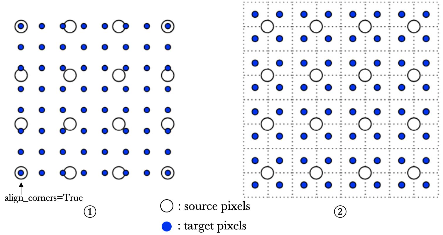
Another convention, "integer corners", or "half-integer centers", puts the origin at the beginning of the signal, so the first pixel is centered at (0.5, 0.5). The two conventions are demonstrated in this figure:
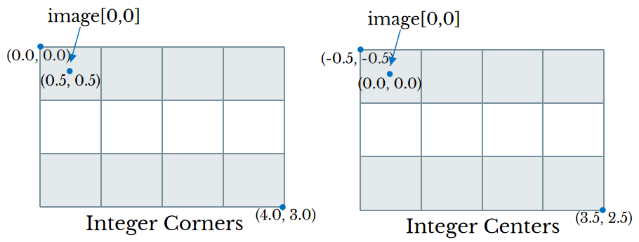
We choose "integer corners", and then will have the following relationship between continuous coordinates and discrete pixel indices:
The choice doesn't matter for resize because absolute coordinates are not part of its API. However, for functions that accept or return absolute coordinates, we should be aware of their convention. For example:
cv2.findContoursreturns integer polygons represented by indices. So we always add 0.5 pixel to its results to obtain coordinates that match our convention.cv2.warpAffineuses "integer centers" and this is complained about in this issue. In fact most OpenCV functions use the "integer centers" convention.pycocotools.mask.frPyObjectsrenders polygons as masks. It accepts polygons in "integer corners" convention. Same forPIL.ImageDraw.polygon, but its results are 0.5 pixel "fatter" due to how its implemented. This has affected cityscapes annotations.RoIAlignin torchvision takes a box in absolute coordinates that match our "integer corners" convention.scipy.ndimage.map_coordinatestakes coordinates in "integer centers" convention.
If a dataset is annotated with coordinates, we also need to know its choice of coordinate system. This information is often not provided by dataset owner, so we make guesses. For example, in COCO it appears that polygon annotations match our convention, but keypoint annotations do not and should be incremented by 0.5.
Now that we have a convention for the coordinate system, it's a good practice in computer vision systems to always use coordinates rather than indices to represent geometries, such as boxes and polygons. This is because indices are integers, and can easily lose precision during geometric operations. Using indices for bounding boxes has caused some issues in Detectron.
Improvements in Detectron & Detectron2
Models in Detectron / Detectron2 all involve localization of objects in images, so the convention of pixels and coordinates matters a lot. Various improvements and bugfixes in the two libraries are related to pixels.
Box Regression Transform
In detection models, bounding box regression typically predicts "deltas" between the ground truth (GT) box and a reference box (e.g. anchor). In training, GT box is encoded to deltas as training target. In inference, the predicted deltas are decoded to become output boxes.
Boxes in Detectron often use integer indices, instead of coordinates. So the width of a
box is given by
|
As innocent as the code seems, the two functions are not inverse of each other: decode(encode(x0, x1)) != (x0, x1).
x1 is incorrectly decoded: it should be center + 0.5 * w - 1 instead.
This bug appeared in the py-faster-rcnn project around 2015, and is still there
today.
It was carried into Detectron and negatively affected results in the Mask R-CNN paper.
Then it's fixed in late 2017
after I found it, and contributed to an improvement of 0.4~0.7 box AP.
Detectron went open source in 2018 with this fix.
In Detectron2, we adopt the rule to always use floating-point coordinates for boxes, so the issue no
longer exists.
Flip Augmentation
How to horizontally flip a geometry? Although pixel indices should be flipped by
Detectron isn't so rigorous on this and it uses
The augmentation library "imgaug" also made this fix.
Delay Conversion to Mask Representation
COCO's instance segmentation data is annotated with polygons that have sub-pixel precision. Converting polygons to binary masks loses the precision due to quantization, and the lost might become more severe during augmentations. Therefore it's preferrable to keep the polygon representation and delay the conversion as much as possible.
In both Detectron and Detectron2, polygon representation are kept during flipping, scaling, and RoI cropping. Masks are not created until the second stage's box predictions are made, where the boxes are used to crop the groundtruth polygons and generate the mask training target.
On the contrary, in TensorFlow's detection code here and here polygons are turned to binary masks immediately at dataset creation time.
Anchor Generation
The code to generate anchors in Detectron is quite long, because it tries to generate integer-valued anchor boxes. By adopting coordinates for all boxes in Detectron2, integer boxes are not needed. This simplifies all the logic to just a few lines of code.
This does not affect accuracy, because the exact values of anchors are not that important as long as the same is used in training & testing.
RoIAlign
The RoIAlign operation crops a region from an image and resize it to certain shape. It's easy to make mistakes because two images and two coordinate systems are involved. Let's derive how to perform RoIAlign.
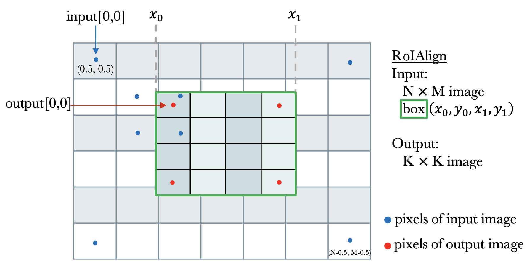
Given an image and a region (the green box), we want to resample a K [i,j] is
sampling_ratio=1).
We show the 4 neighboring input pixels of output[0,0] in the figure.
The indices of 4 nearest pixels of
The original implementation of RoIAlign in Detectron doesn't subtract 0.5 in the end, so it's actually not very aligned. It turns out this detail does not affect accuracy of R-CNNs, because RoIAlign is applied on CNN features, and CNN is believed to be able to fit slightly misaligned features.
However, we have new use cases of RoIAlign in other places, e.g. to crop mask head training targets from the ground truth mask, so
I fixed it in the detectron2 / torchvision RoIAlign with an aligned=True option.
Its unittest
demonstrates how the old version is misaligned.
Btw, once we figured out the coordinate transform formula, it's easy to implement RoIAlign using grid_sample.
This shows that RoIAlign is nothing more than a fused bilinear sampling + averaging.
Using grid_sample is about 10%-50% slower than the RoIAlign CUDA kernel.
Paste Mask
Mask R-CNN is trained to predict masks of fixed resolution (e.g. 28x28) restrained inside given boxes (we call it "RoIMask"). But in the end, we often want to obtain full-image masks. A "paste mask" operation is needed to paste the small RoIMask into the given region in the image.
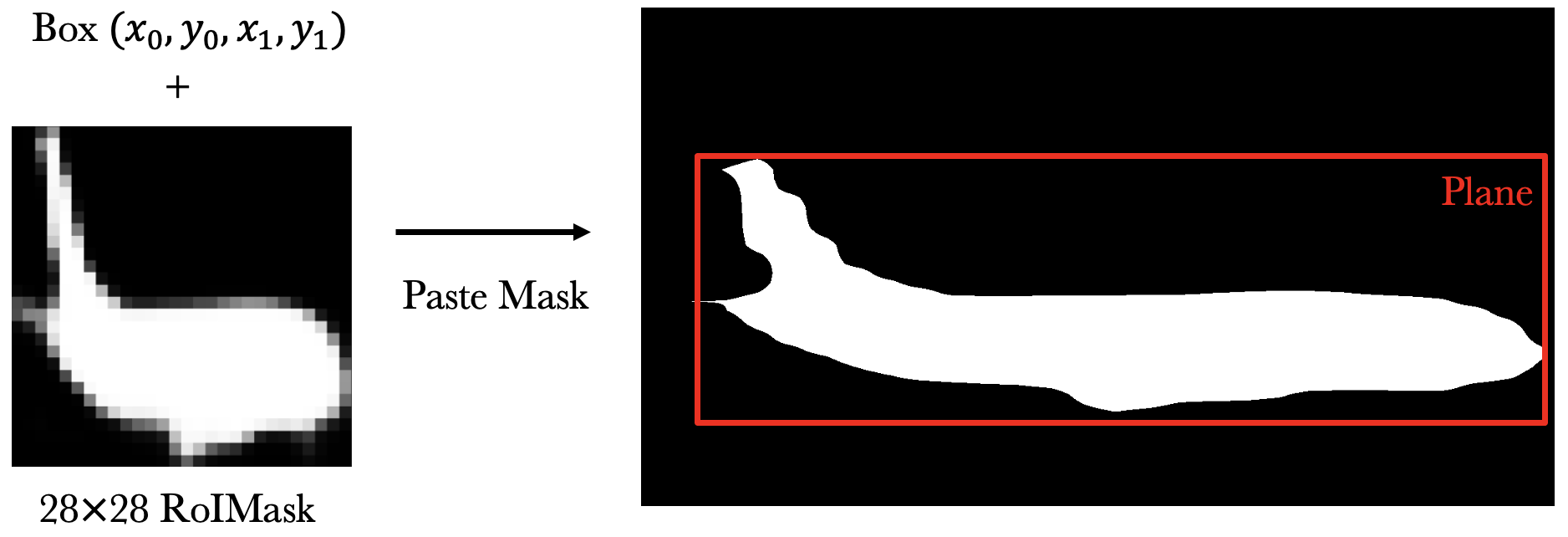
This operation is an inverse of RoIAlign, so it should be implemented similar to our derivation above. In Detectron, this was implemented with some magic rounding & resize that are not exactly the inverse of RoIAlign. Fixing it in detectron2 increases the mask AP by 0.1~0.4.
Point-based Algorithms
Obviously, the paste mask operation can introduce aliasing in the results due to the low resolution RoIMask. This is the motivation behind our work of PointRend.
PointRend is a segmentation method that focuses on point-wise features, where a "point" is not necessarily a pixel, but any real-valued coordinates. Pointly-Supervised Instance Segmentation, also from our team, uses point-wise annotations to train segmentation models. Both projects involve heavy use of point sampling and coordinate transforms. Having a clear and consistent convention of pixels and coordinates was important to their success.
Summary
Due to some sloppy code in the early days of deep learning libraries, today we're facing multiple versions of resize functions. Together with the two different coordinate system conventions, they easily cause hidden bugs in computer vision code.
This article revisits these historical technical debts and shows how these fun details matter in modeling and training. I hope they will help you make proper choices.